It is useful to recall that each coordinate component is just a scalar field. It is a trivial fact, but that is the easiest way to understand what covariant and contravariant vectors really are.

A common way of representing a coordinate system is to draw a grid. A grid is made from the isolines of the coordinate fields, i.e, the \(x\) grid lines are the isolines of \(x\).

If the coordinate system is orthogonal, the \(x\) grid lines are locally tangent to the gradient of the \(y\) field.

Lets take a vector \(\boldsymbol{v}\) in a two-dimensional space. We want \(\boldsymbol{v}\) to represent a spatial quantity which should not depend on the way we measure space.

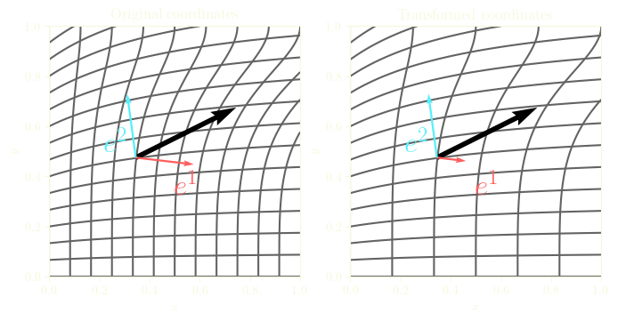
We can use a reference coordinate system, let's say the Cartesian coordinates \((x, y)\) , and the associated vector basis \(\{\boldsymbol{e}_x, \boldsymbol{e}_y\}\).

We can also use another arbitrary coordinate system, with the coordinates \((q^1 , q^2)\), and the vector basis \( \{ \boldsymbol{e}_1, \boldsymbol{e}_2 \} \). This arbitrary coordinate system can be later transformed as we like. We do not know yet how to obtain the vector basis, but it doesn't matter.

The Cartesian coordinates will be used as a reference, i.e., the components of \(\boldsymbol{v}\) will not change in the Cartesian system. Why would we need that? Because otherwise, how would we know that something changed without any reference? But we have yet to create a vector basis in order to express the components of \(\boldsymbol{v}\).

There are two main ways of building a vector basis from a given coordinate system, note that this basis can be local. Let's try both.

Tangent vectors and contravariant components

The most common way to obtain a basis is to take the derivative of the position of a point, \[ \boldsymbol{e}_i = \frac{\partial \vec{r}}{\partial q^i} \]

This yields vectors which are tangent to the other coordinate isolines (isosurfaces in 3D).

The components of \(\boldsymbol{v}\) are written \(v^i\) and thus, \[v = v^1 \boldsymbol{e}_1 + v^2 \boldsymbol{e}_2 \]

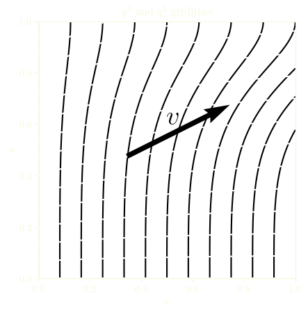
Now, what will happen if we divide the whole field \(q^1\) by two? We can see that the length of \(\boldsymbol{e}_1\) will be multiplied by two.
\(\boldsymbol{v}\) should stay the same, so the component \(v^1\) will be divided by two. That's why the components \(v^i\) are called contravariant (relative to the \(\boldsymbol{e}_i\) basis ), and, \(v^1 \boldsymbol{e}_1 + v^2 \boldsymbol{e}_2\) is called a contravariant vector. Contravariant components are written with upper indices.

Gradient vectors and covariant components

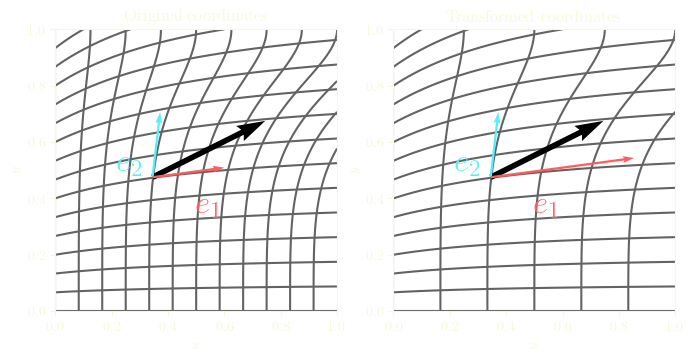
We can use the gradient of each coordinate to build another vector basis for \((q^1, q^2)\), \[\boldsymbol{e}^i = \nabla q^i \]

But how is the gradient defined? We could use our reference Cartesian basis to assess how \((q^1, q^2)\) and \((x, y)\) are related. However, we should not really care, since the gradient field doesn't depend on the coordinate system, and we do not need its expression.

Thus, the vector \(\boldsymbol{v}\) can be written, \[v = v_1 \boldsymbol{e}^1 + v_2 \boldsymbol{e}^2\]

Again, we divide the field \(q^1\) by two. We see that the length of \(\boldsymbol{e}^1\) will also be divided by two. In consequence, the component \(v_1\) has to be multiplied by two. That's the contrary of the previous basis.

So we say that the components \(v_i\) are covariant (relative to the previously described basis, \(\boldsymbol{e}_i\)), and that \(v_1 \boldsymbol{e}^1 + v_2 \boldsymbol{e}^2\) is a covariant vector. Covariant components are written with lower indices.

The names covariant and contravariant are given relative to the \(\boldsymbol{e}_i\) basis. Indeed, if we apply a transform \(M\) to the \(\boldsymbol{e}_i\) basis,

• the contravariant components must undergo the inverse transform, \(M^{-1}\).
• the covariant components must undergo the same transform, \(M\).

Moreover, we see that the basis vectors \(\boldsymbol{e}^i\) are contravariant, and that the \(\boldsymbol{e}_i\) are covariant (relatively to themselves).

The basis for covariant vectors is made from the contravariant vectors \(\boldsymbol{e}^i\). That way the vector \(\boldsymbol{v}\) stays the same after the transformations of \(\boldsymbol{e}_i\).

In the same fashion, the basis for contravariant vectors is made from the covariant vectors \(\boldsymbol{e}_i\).

It should have become clear that the terminology is quite misleading, a vector representing a physical quantity should be the same independently of the way it is written. The terms covariant and contravariant should be used when talking about bases and components. In fact, \(\boldsymbol{e}_i\) and \(\boldsymbol{e}^i\) do not even reside in the same space but this is another story.